
Ultrasound imaging is the same physics whether you are looking inside a patient or inside a weld. A short pulse of sound travels into the body or the material, echoes come back from every boundary and inhomogeneity it meets, and the system turns those echoes into an image. In medicine that might reveal a small lesion or blood flow; in non-destructive testing (NDT) it might reveal a crack, a disbond in a composite, or porosity in a casting.
In both worlds the question is the same: how do we see smaller, fainter things more clearly? The answer is rarely “turn it up”. It lies in how the pulse is designed, how the echoes are captured, and increasingly in the algorithms that turn raw data into images.
What resolution really means
Ultrasound has two main kinds of resolution, and they depend on different things.
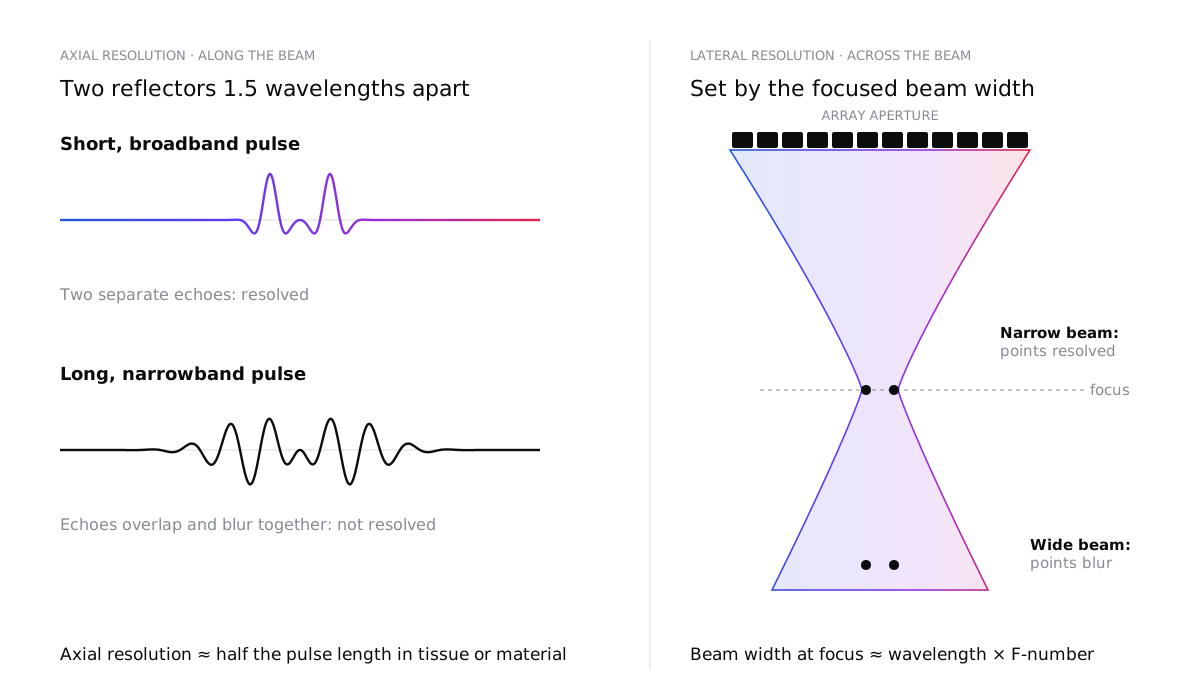
Axial resolution, along the beam, is set by the length of the pulse. Two reflectors can only be separated if their echoes do not overlap, which means axial resolution is roughly half the spatial pulse length. A short pulse needs a wide bandwidth, which is why transducer design and electrical matching matter so much.
Lateral resolution, across the beam, is set by how tightly the beam is focused. At the focus, the beam width is roughly the wavelength multiplied by the F-number (focal depth divided by aperture). A larger aperture or a higher frequency gives a narrower beam, but only near the focus. Our free beam and resolution calculator works out both for your own transducer, from its frequency, bandwidth, aperture and focus.
Higher frequencies improve both, but there is a price: attenuation rises with frequency. In soft tissue it is roughly 0.5 dB per centimetre per megahertz, so a 15 MHz probe that is excellent for skin or tendons cannot reach the depth a 3 MHz abdominal probe can. In NDT, attenuation and scattering depend strongly on the material: fine-grained aluminium is easy, while coarse-grained austenitic steels, cast components and many composites are much harder.
Seeing small changes
Resolution is only half the story. To see a subtle change, it must also stand out from its surroundings: it needs contrast. Echoes come from changes in acoustic impedance, and small or soft targets, such as an early lesion or a tight, closed crack, reflect very little. Meanwhile, countless tiny scatterers in tissue or in a material’s grain structure create speckle: a granular texture that can hide a weak target as effectively as noise.
So the real goal is not just a sharp image, but a high contrast-to-noise ratio: a target that is clearly different from the background, where the “noise” includes speckle and clutter as well as electronic noise.
Why more power can make it worse
When an image looks noisy, the instinct is to transmit more energy. That helps only up to a point.
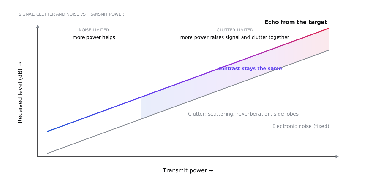
At low power, the image is limited by the electronics’ own noise, and more power genuinely helps. But most of what degrades a real image is clutter, and clutter is made of the same sound you transmitted:
- Scattering from the tissue or grain structure, including multiple scattering in strongly scattering materials.
- Reverberation between layers, such as the skin and fat layers, or the front wall and back wall of a plate.
- Side lobes and grating lobes of the beam, which pick up echoes from directions you are not looking at.
Turn up the power and the clutter rises in step with the signal, so contrast does not improve. Higher pressures also distort the pulse through non-linear propagation, increase heating of the probe and electronics, and, in medicine, run into safety limits. Diagnostic systems are regulated through indices such as the mechanical and thermal index, with limits such as the FDA’s mechanical index of 1.9, and measured outputs do not always match the displayed values.
The better way forward is to make each echo count.
Beamforming: focusing with time
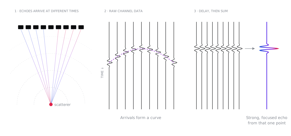
An array transducer is made of many small elements. Beamforming uses precisely timed delays to steer and focus the sound, both when transmitting and when receiving.
The workhorse is delay-and-sum (DAS). For every point in the image, the system calculates how long the echo from that point takes to reach each element, shifts each channel by that delay, and adds them up. Echoes from the chosen point add coherently into a strong signal; echoes from elsewhere add incoherently and partly cancel.
Modern systems refine this in many ways. Dynamic receive focusing updates the delays continuously with depth. Apodization weights the elements to lower the side lobes, at the cost of a slightly wider main beam. Beyond that, there is a whole family of methods, each with its own trade-offs:
| Method | Strengths | Limitations |
|---|---|---|
| Delay-and-sum | Robust, fast, well understood | Side lobes and clutter limit contrast |
| Synthetic aperture / full matrix capture with TFM | Focused everywhere in the image, excellent resolution; widely used in NDT | Large data volumes and heavy computation |
| Plane-wave or diverging-wave compounding | Hundreds to thousands of images per second | Needs many angles for full quality; sensitive to motion |
| Adaptive beamforming (e.g. minimum variance) | Sharper lateral resolution | Computationally expensive; can alter speckle statistics |
| Coherence-based methods (coherence factor, DMAS, SLSC) | Strong clutter suppression, better contrast | Can suppress weak true echoes; non-linear and harder to quantify |
| Learned (AI) beamformers | Fast; can learn complex corrections | Need representative training data; harder to validate and generalise |
There is no single best algorithm. The right choice depends on the tissue or material, the depth, the frame rate you need, your computing budget and, for medical devices, how the method will be validated.
Time domain or frequency domain?
Image reconstruction can be done in two broad ways.
Time-domain methods such as delay-and-sum work directly with the echo signals. They handle almost any array geometry and can account for varying speed of sound, layers and wedges, but their computational cost grows with the number of image points and channels.
Frequency-domain methods, such as Fourier or wavenumber (f-k) migration borrowed from seismic imaging, transform the data with fast Fourier transforms and reconstruct whole images at once. They can be dramatically faster, but they assume a uniform, or neatly layered, medium.
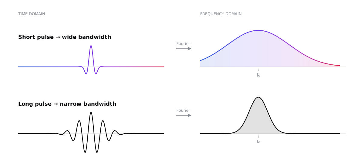
The same duality explains why the pulse matters so much. A pulse that is short in time is broad in frequency, and a long pulse is narrow in frequency.
Making the invisible visible: the signal chain
Many of the biggest improvements in image quality come from details along the signal chain, long before any clever algorithm.
Pulse bandwidth and centre frequency. These come from the transducer’s design, its matching layers and backing, and its electrical impedance matching. Wider bandwidth gives shorter pulses and better axial resolution.
Sample rate. The Nyquist criterion is only the starting point. Beamforming needs accurate delays, so systems typically sample at several times the centre frequency, or interpolate finely between samples. Demodulating to baseband (IQ data) then keeps the data rate manageable.
Filtering. Band-pass and matched filters remove out-of-band noise. Time-gain compensation corrects for attenuation with depth. Harmonic imaging listens for echoes at twice the transmitted frequency, generated as the pulse travels. Because harmonics build up away from the near-field layers, they carry less reverberation and clutter, which gives cleaner images in difficult cases.
Pulse modulation and coded excitation. Instead of a short spike, the system can transmit a longer, coded waveform such as a frequency sweep (chirp) or complementary codes. A matched filter on receive compresses it back into a short pulse.
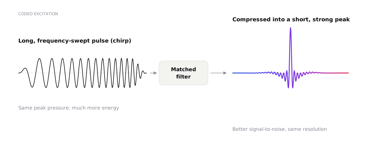
The result is a better signal-to-noise ratio, and more penetration, without a higher peak pressure, with resolution set by the bandwidth. It needs care: imperfect compression creates range side lobes, and non-linear effects and frequency-dependent attenuation distort the code. In NDT, coded excitation is valuable for highly attenuating materials; in medicine, it helps reach deeper while staying within safety limits.
Compounding and averaging. Combining images taken from different angles or frequency bands reduces speckle and reveals continuous boundaries more clearly.
Computational ultrasound is the future
For decades, image formation was locked into fixed hardware. Today, more and more systems capture the raw data from every channel and form images in software, on GPUs. That changes what is possible:
- Ultrafast imaging at thousands of frames per second, enabling shear-wave elastography, sensitive blood-flow imaging and functional imaging of the brain.
- Super-resolution imaging: by tracking individual microbubbles, ultrasound localization microscopy can map microvessels far smaller than the classical diffraction limit.
- Model-based and adaptive reconstruction that estimates the local speed of sound and corrects for aberration from fat layers, bone or complex part geometries.
- Full matrix capture with the total focusing method in NDT, giving images focused everywhere, with better characterisation of small and complex flaws.
- Machine learning for beamforming, denoising and interpretation, provided it is trained on representative data and validated with the rigour medical and safety-critical applications demand.
The common thread is that the transducer, the electronics and the algorithms are designed together, as one system. The best results come from choosing the pulse, the array, the sampling and the reconstruction to suit the question being asked, rather than optimising each in isolation.
Choosing the right approach
If you are developing an imaging system, medical or industrial, start with the questions that matter:
- What is the smallest feature or change you need to detect, and at what depth? This sets the frequency, aperture and bandwidth.
- What limits you today: electronic noise or clutter? The answer decides whether you need more signal or better rejection.
- What frame rate and computing budget do you have? This guides the choice of beamformer.
- How will you validate it? Especially for medical devices, the reconstruction method is part of what must be verified.
We design ultrasound transducers, imaging systems and signal-processing pipelines for medical and industrial applications, from acoustic simulation to working prototypes. If you are trying to see something that is currently invisible, let’s talk.